

RCBD vs CRD
Split Plot (Tillage)
Contrasts (orthogonal contrast
coefficients) (Table on line)
Contrasts for Unequal Treatment Spacing ( proc iml )
Run equally spaced rates in IML and see what it generates?
| Treatment | N rate | Tillage |
| lb/ac | ||
| 1 | 0 | zero |
| 2 | 50 | zero |
| 3 | 100 | zero |
| 4 | 150 | zero |
| 5 | 0 | conv |
| 6 | 50 | conv |
| 7 | 100 | conv |
| 8 | 150 | conv |
| CRD | CRD | RCBD | RCBD-(split) | ||||
| Source of variation | df | Source of variation | df | Source of variation | df | Source of variation | df |
| Total (4*8)-1 | 31 | Total (4*8)-1 | 31 | Total (4*8)-1 | 31 | Total (4*8)-1 | 31 |
| block | 3 | block | 3 | ||||
| treatment | 7 | treatment (8-1) | 7 | treatment (8-1) | 7 | tillage | 1 |
| Tillage | 1 | block*tillage | 3 (a) | ||||
| Nrate | 3 | nrate | 3 | ||||
| nrate*tillage | 3 | nrate*tillage | 3 | ||||
| error | 24 | error | 24 | error | 21 | error | 18 (b) |
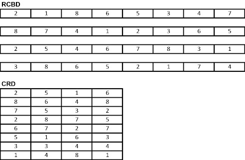
| RCBD-(no split) | zero till | conv. Till | ||||||
| Rep 1 | 1 | 8 | 3 | 2 | 5 | 4 | 7 | 6 |
| Rep 2 | 6 | 2 | 7 | 8 | 3 | 1 | 5 | 4 |
| Rep 3 | 3 | 6 | 1 | 4 | 8 | 5 | 2 | 7 |
| Rep 4 | 7 | 4 | 2 | 5 | 6 | 8 | 3 | 1 |
| RCBD (split block) | zero till | conv. Till | ||||||
| Rep 1 | 1 | 4 | 3 | 2 | 5 | 8 | 7 | 6 |
| Rep 2 | 6 | 5 | 7 | 8 | 2 | 1 | 3 | 4 |
| Rep 3 | 2 | 3 | 1 | 4 | 8 | 5 | 6 | 7 |
| Rep 4 | 7 | 8 | 6 | 5 | 4 | 2 | 3 | 1 |
| Factorial Arrangement of Treatments | vs | "Factorial Experimental Design" | |||||
| Needed when little is known about the interaction | |||||||
| Main Effects | Levels | Value | Treatment Structure | ||||
| N rates | 3 | 0, 40, 80 | Trt. | N rate | P rate | Legume | |
| P rates | 3 | 0, 10, 20 | 1 | 0 | 0 | Y | |
| Legume Cover | 2 | Y, N | 2 | 40 | 0 | Y | |
| 3 | 80 | 0 | Y | ||||
| Trt's | 18 | 4 | 0 | 10 | Y | ||
| 5 | 40 | 10 | Y | ||||
| Danger of having too many levels | 6 | 80 | 10 | Y | |||
| 7 | 0 | 20 | Y | ||||
| 8 | 40 | 20 | Y | ||||
| 9 | 80 | 20 | Y | ||||
| 10 | 0 | 0 | N | ||||
| 11 | 40 | 0 | N | ||||
| 12 | 80 | 0 | N | ||||
| 13 | 0 | 10 | N | ||||
| 14 | 40 | 10 | N | ||||
| 15 | 80 | 10 | N | ||||
| 16 | 0 | 20 | N | ||||
| 17 | 40 | 20 | N | ||||
| 18 | 80 | 20 | N | ||||
? Incomplete Factorial Treatment Structure ?
data one;
input rep nrate legume $ yield preP;
cards;
1 0 L 16 16
1 50 L 25 13
1 100 L 29 9
1 150 L 35 8
1 0 NL 35 18
1 50 NL 35 6
1 100 NL 38 9
1 150 NL 39 19
2 0 L 20 22
2 50 L 26 23
2 100 L 30 28
2 150 L 32 25
2 0 NL 36 4
2 50 NL 36 8
2 100 NL 37 6
2 150 NL 40 7
3 0 L 17 8
3 50 L 22 19
3 100 L 25 48
3 150 L 29 22
3 0 NL 29 23
3 50 NL 34 25
3 100 NL 38 24
3 150 NL 40 18
proc print;
proc glm;
class rep legume nrate;
model yield = rep legume nrate legume*nrate;
contrast 'Nrate_lin' nrate -3 -1 1 3;
contrast 'Nrate_quad' nrate 1 -1 -1 1;
contrast 'legume*nrate_lin' legume*nrate -3 -1 1 3 3 1 -1 -3;
contrast 'legume*nrate_quad' legume*nrate 1 -1 -1 1 -1 1 1 -1;
means nrate legume legume*nrate;
run;
| Legume (1) | No Legume(-1) | ||||||
| 0 | 50 | 100 | 150 | 0 | 50 | 100 | 150 |
| linear | |||||||
| -3 | -1 | 1 | 3 | 3 | 1 | -1 | -3 |
| quadratic | |||||||
| 1 | -1 | -1 | 1 | -1 | 1 | 1 | -1 |
Is it important to identify/discuss an interaction if it exists? (MSE's over sites?)
Antagonistic Interaction
Synergistic Interaction (did they respond the same)
model yield = rep legume rep*legume nrate nrate*legume;
test h = rep legume e = rep*legume;
means legume nrate nrate*legume;
Weaknesses of the split plot is the power in testing the difference in having a legume/or not because the rep*legume must be used as the error term.
----------------------------------------------------------------------------------------------
Factorial Arrangement of Treatments (xx factorial design xx )
Tillage 2 N Rates 4 Factorial Treatment Structure = 2 * 4 = 8 total treatments
All levels of N Rates evaluated over all levels of Tillage
Factorial treatment structure allows for testing the interaction between the two ( or nrate*tillage )
? Did N rates respond the same for the two different tillage systems ?
? This is the value of the factorial treatment structure ? BUT.... does it use up too many treatments
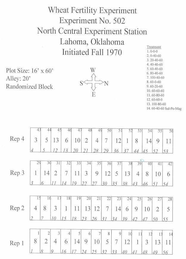
| Efficient Design | ||||||||
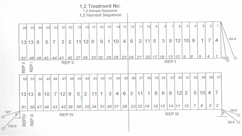
| 4 reps | df | 3 reps | df | |||||
| Replications | 4 | Total | (4*13)-1 | 51 | (3*13)-1 | 38 | ||
| Treatments | 13 | Rep | 4 - 1 | 3 | 3 -1 | 2 | ||
| Trt | 13-1 | 12 | 13-1 | 12 | ||||
| Factorial Arrangement of Treatments | Error | 36 | 24 | |||||
| 4 | Rate | |||||||
| 3 | X-var. | 12 | ||||||
| 1 | check | 13 | ||||||
| RCBD | Randomized Complete Block Design | |||||||
| CRD | Completely Random Design | |||||||

If the World were 100 People?
6.7 % hold college degree's
Linear Interaction
Contrast Program for Unequal Spacing
proc iml;
dens={0 100 600 1200}; **
p=orpol(dens);
t=nrow(p);
do i=1 to t;
pr=abs(p[,i]);
pr[rank(abs(p[,i]))]=abs(p[,i]);
do j=t to 1 by -1;
if pr[j] > 1.e-10
then scale=pr[j];
if abs(p[j,i]) <
1.e-10 then p[j,i]=0;
end;
p[,i]=p[,i]/scale;
end;
print p;
run;
The only thing that needs to be changed is the trt values.
Output
Trt P lin quad cubic
0 1 -3.8 19.416667 -11
100 1 -3 1 14.4
600 1 1 -40.66667 -4.4
1200 1 5.8 20.25 1
data one;
input rep trt buac;
cards;
1 1 20.78765244
1 2 35.3777439
1 3 41.24329268
1 4 .
1 5 42.1839939
1 6 62.49207317
1 7 59.35640244
1 8 40.00746951
1 9 52.97439024
1 10 18.24222561
1 11 59.55929878
1 12 46.51859756
1 13 34.97195122
2 1 19.44115854
2 2 24.73490854
2 3 37.11158537
2 4 63.98612805
2 5 41.9257622
2 6 46.38948171
2 7 38.9929878
2 8 31.06158537
2 9 53.93353659
2 10 18.62957317
2 11 48.76890244
2 12 49.43292683
2 13 41.53841463
3 1 21.04588415
3 2 30.17621951
3 3 47.58841463
3 4 41.35
3 5 47.82820122
3 6 41.0035061
3 7 .
3 8 37.09314024
3 9 41.48307927
3 10 13.53871951
3 11 57.3089939
3 12 49.67271341
3 13 30.12088415
4 1 18.96158537
4 2 23.70198171
4 3 39.25121951
4 4 54.35777439
4 5 34.3632622
4 6 50.22606707
4 7 28.09192073
4 8 30.82179878
4 9 25.82317073
4 10 14.64542683
4 11 43.2722561
4 12 20.49253049
4 13 28.18414634
proc print;
proc glm;
class rep trt;
model buac = rep trt;
means trt;
run
;proc mixed; class rep trt;
model buac = trt/ddfm=satterth;
random rep;
lsmeans trt/diff;
run;
quit
;
input rep trt buac gn;
cards;
1 1 29.88109756 1.970387936
1 2 32.0945122 1.914626837
1 3 53.95198171 1.851969123
1 4 50.35518293 1.821092963
1 5 71.93597561 1.963828087
1 6 80.78963415 2.209946632
1 7 88.8132622 2.672821283
1 8 70.27591463 2.546777248
1 9 73.31935976 2.218581676
1 10 83.27972561 2.157410383
1 11 73.04268293 2.675846577
1 12 97.94359756 2.663606405
1 13 71.38262195 .
1 14 76.63948171 2.125741243
2 1 22.6875 1.89458847
2 2 39.56478659 1.776858568
2 3 44.26829268 1.875116944
2 4 73.59603659 2.396464348
2 5 69.9992378 1.872512221
2 6 98.77362805 2.288419008
2 7 84.93978659 2.727875233
2 8 74.14939024 2.210676908
2 9 90.47332317 2.218745947
2 10 97.11356707 2.209470749
2 11 87.15320122 2.309687138
2 12 97.66692073 2.404773235
2 13 77.74618902 2.741914749
2 14 95.73018293 2.243032694
3 1 32.0945122 1.838460803
3 2 38.7347561 1.839552999
3 3 63.08231707 1.93320477
3 4 74.42606707 1.997364521
3 5 73.31935976 2.284578085
3 6 91.85670732 2.508112431
3 7 85.76981707 2.434265614
3 8 91.58003049 2.200210571
3 9 72.48932927 2.121579409
3 10 96.00685976 2.188293457
3 11 86.87652439 0.002466053
3 12 78.57621951 2.470286846
3 13 71.93597561 3.035435438
3 14 88.25990854 2.087241888
4 1 36.79801829 1.906446576
4 2 48.14176829 2.077796221
4 3 57.54878049 1.905510187
4 4 72.7660061 2.263180017
4 5 87.70655488 2.21556139
4 6 85.49314024 2.750952721
4 7 93.79344512 2.628683805
4 8 81.89634146 2.195582151
4 9 93.79344512 2.303760767
4 10 89.08993902 2.525472641
4 11 89.64329268 2.401524544
4 12 100.1570122 2.290474653
4 13 68.33917683 2.729845285
4 14 96.00685976 2.053695917
proc print;
data two; set one;
gnuptake = (buac*60)*(gn/100);
proc glm data = two;
class rep trt;
model buac gn gnuptake = rep trt;
contrast '1-5 versus 6,7' trt 1 1 1 1 1 -2.5 -2.5 0 0 0 0 0 0 0;
contrast '1-5 versus 6,7' trt 1 1 1 1 1 -2.5 -2.5;
contrast '2-5 versus 6,7' trt 0 1 1 1 1 -2 -2;
means trt;
lsmeans trt;
run;