 RM
2013
RM
2013Estimated probabilities (reliabilities) of treatment
(any treatment where a direct comparison can be made with a check) response
compared to a check for the sample of treatment differences (years or
locations) can be determined as defined by Eskridge and Mumm (1992) where:
RNi = P(Z > - ydi/sdi) such that Z is a standard normal random variable and
ydi and sdi are estimates of the sample mean difference and standard
deviation, respectively.
A
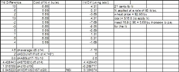
modified reliability estimate (economic reliability, REi) can be calculated
by subtracting the costs (in yield units) of the fertilizer and its
application from the mean difference for the ith treatment (di) against the
treatment check as: REi = P(Z > -(ydi - ci)/ sdi) where ci represents the
equivalent yield necessary to pay for the fertilizer and its application for
a given price ratio.
These
values are then substituted in the equation to calculate reliability for
normally distributed differences.
The recalculated reliability represents the normal probability that a
treatment will outperform the treatment check in a quantity superior to ci,
therefore, providing an estimate of the economic feasibility of the practice
as well as allowing direct comparisons of net benefits among calculated
reliabilities for a given price ratio.

libname lib2 'c:\temp';
data one;
input x y z;
filename grafout 'c:\temp\surf.gsf';
goptions nodisplay gsfmode=replace device=hpljs2
GSFNAME=GRAFOUT gwait=15 fby=xswiss hby = 1.75 gouttype=dependent;
title f=xswiss 'Surface Model';
proc rsreg data = one out = two;
model z = x y /predict;
proc g3grid data = two out = three;
grid x*y=z/spline;
proc g3d data = three gout=new;
plot x*y=z;
run;
Procedure for Determining
Differences in Population Means
cards;
1
A
6.17
21.47
0.924
150
2
A
6.27
18.69
0.939
139
3
B
6.16
21.20
1.042
142
4
B
5.65
41.74
1.054
144
proc ttest;
classes time;
var ph p k oc;
run;
Randomized Complete Block
Randomization
Title ' RCBD 3 reps, 13 treatments';
proc plan seed = 37275;
factors blocks = 3 ordered trts = 13;
run;
Program to output Transposed Data
data one;
Input yr trt yield;
Cards;
88
1
1000
88
2
2000
88
3
2400
89
1
4000
89
2
3200
89
3
3500
data two; set one;
proc sort; by trt yr;
proc transpose data = two out = three prefix = y ;
id yr;
var yield;
by trt;
proc print;
run;
Contrast Program for Unequal
Spacing
dens={0 100 600 1200}; **
p=orpol(dens);
t=nrow(p);
do i=1 to t;
pr=abs(p[,i]);
pr[rank(abs(p[,i]))]=abs(p[,i]);
do j=t to
1 by -1;
if pr[j] > 1.e-10 then scale=pr[j];
if abs(p[j,i]) < 1.e-10 then p[j,i]=0;
end;
p[,i]=p[,i]/scale;
end;
print p;
run;
The only thing that needs to be
changed is the trt values.
Output
Trt
P
lin
quad
cubic
0
1
-3.8
19.416667
-11
100
1
-3
1
14.4
600
1
1
-40.66667
-4.4
1200
1
5.8
20.25
1
Test of Differences in Slope and
Intercept Components from Two Independent Regressions
input exp x y;
if exp = 1 then intc_dif = 0;
if exp = 2 then intc_dif = 1;
slop_dif = intc_dif*x;
cards;
1
3.31878
45.8971
1
3.31716
45.24701
1
3.31162
42.59693
2
3.26607
54.4
2
3.32216
40.7
2
3.31122
55.7
data two; set one;
proc sort; by exp;
proc reg;
model y = x intc_dif slop_dif;
run;
proc reg;
by rep;
model y = x;
run;
input rep
trt x
y;
cards;
proc nlin data = one best = 3;
parms b0=200 to 400 by 20 b1=-
if x<njoint then do;
model y = b0 + b1*x;
der.b0=1;
der.b1=x;
der.njoint=0;
end;
else do;
model y=b0+b1*njoint;
der.b0=1;
der.b1=njoint;
der.njoint=b1;
end;
file print;
if _obs_ =1 and _model_ =0 then do;
plateau = b0 + b1*njoint;
put plateau=;
end;
plateau=b0+b1*njoint;
id plateau;
output out = new p = pry parms=b0 b1 njoint sse=sse;
run;
proc plot;
plot y*x='+' pry*x='*'/overlay;
run;
proc means noprint;
var y sse b0 b1 njoint plateau;
output out = new2 n = tdf
mean = y sse b0 b1 njoint plateau
css=csst;
data new3; set new2;
intercpt=b0; slope=b1; joint=njoint;
rsq=(csst-sse)/csst;
edf=tdf-3;
ssr=csst-sse;
msr=ssr/2;
mse=sse/edf;
f=msr/mse;
probf=1-(probf(f,2,edf));
keep intercpt slope joint plateau rsq f probf;
proc print;
run;
input rep
trt x
y;
cards;
proc nlin data = one best = 2;
parms b0=50 to 100 by 10 b1=-0.5 to -0.1 by 0.01
joint=10 to 50 by 10
b2 = -.5 to .1 by 0.05;
if x<joint then do;
model y = b0 + b1*x;
der.b0=1;
der.b1=x;
der.joint=0;
der.b2=0;
end;
else do;
model y=b0+(b1-b2)*joint+b2*x;
der.b0=1;
der.b1=joint;
der.joint=b1-b2;
der.b2=x-joint;
end;
file print;
if _obs_ =1 and _model_ =0 then do;
joinlev = b0 + b1*joint;
put joinlev=;
end;
joinlev=b0+b1*joint;
id joinlev;
output out = new p = pry parms=b0 b1 joint b2 sse=sse;
run;
proc plot;
plot y*x='+' pry*x='*'/overlay;
run;
proc means noprint;
var y sse b0 b1 joint b2 joinlev;
output out = new2 n = tdf
mean = y sse b0 b1 joint b2 joinlev
css=csst;
data new3; set new2;
intercpt=b0; slope=b1; joint=joint; slope2=b2;
jresp=joinlev;
rsq=(csst-sse)/csst;
edf=tdf-4;
ssr=csst-sse;
msrg=ssr/3;
mse=sse/edf;
f=msrg/mse;
probf=1-(probf(f,2,edf));
keep intercpt slope joint slope2 joinlev rsq msrg mse
edf f probf;
proc print;
run;
Experiment:
Influence of Nitrogen Rate and Mowing Height on Sensor Based
Detection of Nutrient Stress
lb N/1000 ft2/month
inches
__________________________________________
1
0
0.5
2
0.5
0.5
3
1.0
0.5
4
1.5
0.5
5
0
1.5
6
0.5
1.5
7
1.0
1.5
8
1.5
1.5
__________________________________________
Replications: 4
Experimental design: CRD
CRD
CRD
RCBD
Source of variation
df
Source of variation
df
Source of variation
df
Total (4*8)-1
31
Total (4*8)-1
31
Total (4*8)-1
31
block
3
height
1
treatment
7
treatment
7
nrate
3
nrate*height
3
error
24
error
24
error
21
proc glm;
classes height nrate;
model yield = nrate height nrate*height;
contrast 'Nrate_lin' nrate
-3 -1 1 3;
contrast 'Nrate_quad' nrate
1 -1 -1 1;
contrast 'Nrate_cub' nrate
-1 3 -3
1;
contrast 'height*nrate_lin' height*nrate
-3 -1 1 3 3 1 -1 -3;
contrast 'height*nrate_quad' height*nrate 1 -1 -1 1 -1
1 1 -1;
means nrate height nrate*height;
run;
height
0.5
1.5
____________________________
_____________________________
0
0.5
1.0
1.5
0
0.5
1.0
1.5
height
0.5
1.5
1
-1
____________________________
_____________________________
nrate
(linear)
0
0.5
1.0
1.5
0
0.5
1.0
1.5
-3
-1 1 3 -3 -1 1 3
interaction
coefficients (height*nrate_lin)
-3
-1
1
3
3
1
-1
-3

