

SAS Programs
Several Programs including Linear Plateau, Surface Response, etc.
Split Plot in Space (using depth as the non-random split)
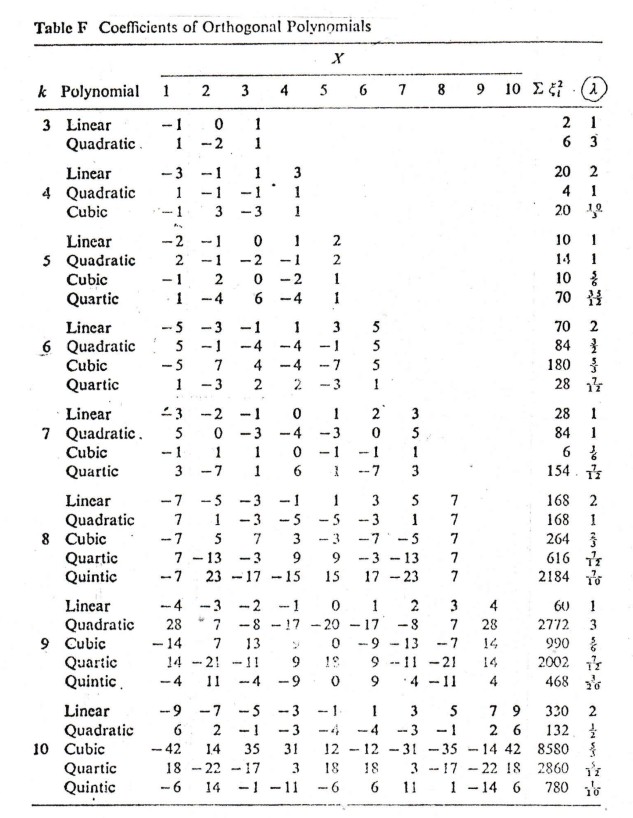
Contrast Coefficients (equally spaced)
Contrast coefficients (un equally spaced) (PROC IML)
Stability Analysis
Long Term Experiment Design and Analysis
Lahoma 502 Data Base
Lahoma 502 Plot Plan
Lahoma 502 (NH4 and NO3 by depth) (lah50288.sas)
Soil-Plant Buffering of Inorganic Nitrogen in Continuous Winter Wheat.
Agron J 1995 87: 827–834
Linear Plateau, and Plateau Linear
options linesize = max pagesize = max; (data lines very long)
Plot Plan
title 'RCBD 3 reps, 13 treatments';
proc plan seed =37275;
factors blocks=3 ordered trts =13;
run;
title 'RCBD 5 reps, 7 treatments 2 Beds';
proc plan seed =37275;
factors blocks=5 beds = 2 ordered trts =7;
run;
title 'CRD, 4 trts, 3
reps';
data a;
do unit=1 to 12;
if (unit<=3) then treat=1;
if (unit>3<6) then treat=2;
if (unit>6<9) then treat=3;
if (unit>9<12) then treat=4;
output;
end;
proc plan seed=37255;
factors unit=12;
output data=a out =b;
proc sort; by unit;
proc print;
run;
Output MEANS to a NEW DATA SET
1. proc sort; by seedwt drum;
proc means noprint data = two; var hindex single; by
seedwt drum;
output out = new2 mean= mhindex msingle;
proc print data = work.new2;
seedwt = seed weight
drum = hand planter drum
hindex (new index developed using singles, multiples,
and blanks)
2. proc sort; by yr trt;
proc means noprint data = two; var mgha buac;
output out = new2 mean = mmgha mbuac; by yr trt;
proc print data = work.new2;
run;
#1 Output Sum of Rain (added variable) and Temp (averaged value) by Month and Year and THEN Merged (rain and temp) by Month and Year
data one;
input yr month day Loc $ temp rain;
cards;
.......
data two; set one;
tempC = (temp -32)*5/9;
proc sort; by yr month;
proc means noprint data = two; var tempc;
output out = new2 mean = mtempc ; by yr month;
proc print data = work.new2;
run;
proc summary data=one nway;
class yr month;
var rain;
output out = new3 sum = sum_rain;
run;
proc print data = new3;
run;
data three; set new2;
proc sort; by yr month;
data four; set new3;
proc sort; by yr month;
data five; merge new2 new3; by yr month;
proc print;
run;
#2 Output Sum of Rain (added variable) and Temp (averaged value) by Month and Year and THEN Merged (rain and temp) by Month and Year
proc summary data=one nway;
class yr month;
var rain;
output out = nrain sum = sum_rain;
data two; set one;
proc summary data = two nway;
class yr month;
var temp;
output out = ntemp mean(temp) =mean_temp;
data three; set nrain; proc sort; by yr month;
data four; set ntemp; proc sort; by yr month;
data five; merge three four; by yr month;
proc print data = five;
FOR generating output that was within GLM (MSE, etc.)
3. data two; set one;
proc sort; by yr;
proc glm data = two;
class rep trt;
model yield = rep trt; by yr;
output out = work.stat1 p=yP0 r=rmse stdr=ervar;
proc means noprint data =work.stat1; var yp0 rmse
ervar ; by yr;
output out = new2 mean = myp0 mrmse mervar;
proc print data = new2;
run;
Testing for a Normal Distribution (2011, 502 data, GN, buac, NDVI)
data one;
input rep trt buac gn ndvi;
cards;
1 1 29.13 1.9456 0.451165
1 2 22.44 1.8788 0.40397
1 3 37.07 1.8926 0.53212
1 4 34.88 1.9351 0.527
1 5 38.15 2.2403 0.634425
1 6 35.15 2.1966 0.67538
1 7 34.83 2.7993 0.7433
1 8 48.58 2.5252 0.65529
1 9 35.77 2.1586 0.57059
1 10 37.86 2.4264 0.627675
1 11 47.26 2.9479 0.69157
1 12 48.48 2.6666 0.758295
1 13 47.89 2.6558 0.769345
1 14 38.62 2.3973 0.63071
2 1 25.52 1.7441 0.430055
2 2 29.42 1.6768 0.468865
2 3 30.32 1.83 0.48483
2 4 41.71 2.1317 0.58317
2 5 45.88 2.3133 0.670615
2 6 47.45 2.4608 0.751955
2 7 48.13 2.9647 0.7962
2 8 41.68 2.1915 0.63959
2 9 49.90 2.4681 0.672735
2 10 42.09 2.2705 0.65098
2 11 47.43 2.2011 0.655445
2 12 50.31 2.4045 0.696805
2 13 46.97 3.0859 0.782475
2 14 47.57 2.7973 0.71301
3 1 33.32 1.8448 0.544005
3 2 29.50 1.92 0.542
3 3 24.72 1.7563 0.521975
3 4 41.12 2.1688 0.65147
3 5 23.69 2.6932 0.72394
3 6 50.76 2.8365 0.737355
3 7 54.57 2.6516 0.8103
3 8 45.64 2.4243 0.714515
3 9 24.64 2.3779 0.697485
3 10 48.06 2.4276 0.687275
3 11 53.34 2.4215 0.74007
3 12 21.19 2.8484 0.687465
3 13 17.13 3.4241 0.80911
3 14 46.13 1.8807 0.73776
4 1 29.12 1.9349 0.53002
4 2 28.70 2.1478 0.56066
4 3 29.06 1.8011 0.570915
4 4 27.45 2.1518 0.661675
4 5 33.33 2.2393 0.698135
4 6 28.41 2.8012 0.774795
4 7 41.24 3.019 0.81976
4 8 44.58 2.4654 0.71015
4 9 48.67 2.5505 0.764265
4 10 31.52 2.3874 0.75282
4 11 46.24 2.1883 0.70825
4 12 40.51 2.1445 0.74003
4 13 33.24 2.7976 0.794645
4 14 46.06 2.3416 0.75745
title '2011 502 data';
proc univariate normal plot;
var buac gn ndvi;
proc chart;
vbar buac;
proc chart;
vbar gn;
proc chart;
vbar ndvi;
run;
Delete Function
If 1 <TRT<10 then delete;
(gets rid of trts 2-9 and keeps 1, 10, 11, 12, 13)
Transpose
Function, OUTPUT DATA (2 examples)
data one;
input yr trt yield;
cards;
88 1 1000
88 2 2000
88 3 2400
89 1 4000
89 2 3200
89 3 3500
92 1
6000
92 2
7200
92 3
8800
data two; set one;
proc sort; by trt yr;
proc transpose data = two
out = three prefix = y ;
id yr;
var yield;
by trt;
proc print;
run;
data one;
input YR TRT BUAC;
cards;
1893	1	10.5
1893	2	10.5
1894	1	20.9
1894	2	20.9
data two; set one;
if trt <3 then delete;
if trt >4 then delete;
data three; set two;
proc sort; by yr trt;
proc means noprint; by yr trt; var buac;
output out = new mean = ybuac;
data new1; set new; proc sort; by yr;
proc transpose data = new1 out = three prefix = trt;
by yr;
id trt;
var ybuac;
proc print;
run;
Procedure for Determining Differences in Population
Means
data one; input sample
time $ ph P oc k;
cards;
1 A
6.17 21.47 0.924 150
2 A
6.27 18.69 0.939 139
3 B
6.16 21.20 1.042 142
4 B
5.65 41.74 1.054 144
proc ttest;
class time;
var ph oc;
run;
COMPOSITE PROGRAM SIMPLE STATISTICS
A. Proc Corr (r values) (see added proc procedures that go with this data set)data one;
input ndvi buac gn ph sn sp;
cards;
0.6205 34.42627 2.5107 6.39 0.10469 32.80725
0.294 18.51818 2.59762 5.54 0.0788 2.52685
0.429 24.41195 2.2206 5.40 0.0756 42.48705
0.4335 35.67636 2.6788 5.00 0.09356 28.1535
0.413 37.01768 2.8313 4.79 0.08893 44.907
0.5675 39.72107 2.8135 4.99 0.09549 35.04105
0.62347 19.14847 2.2536 6.48 0.08441 35.6701
0.290535 6.427076 2.1697 5.43 0.0715 6.8042
0.31301 8.449443 1.9589 5.44 0.06613 46.92191
0.684435 23.14757 2.5939 4.86 0.08623 50.63324
0.713725 23.81803 2.5314 4.75 0.07685 56.93661
0.7247 24.93252 2.8309 5.14 0.07576 46.68627
0.736 39.52 1.9444 6.55 0.08145 43.52569
0.286 15.22 1.7883 5.40 0.052864 7.91341
0.389 19.41 1.5578 5.32 0.05636 68.54739
0.661 44.37 1.7588 4.72 0.08549 56.56025
0.666 46.67 1.7828 4.64 0.06896 51.67229
0.740 44.76 1.9573 5.18 0.07717 43.06017
0.490 42.56 1.791567 6.19 0.096 81.34
0.227 15.32 1.674467 5.3 0.063 10.47
0.302 22.68 1.562867 5.18 0.073 76.86
0.417 52.08 1.670433 4.75 0.098 79.98
0.392 49.43 1.608467 4.57 0.095 88.72
0.441 53.15 1.674 5.12 0.101 73.85
0.44595 33.38476 . 6.61 0.146 104.96
0.24467 17.2852 . 5.56 0.123 21.45
0.29489 17.78717 . 5.39 0.136 119.75
0.33835 32.95005 . 4.91 0.16085 99.12
0.31672 31.94973 . 4.74 0.18162 88.43
0.38775 35.20741 . 5.44 0.16518 110.3
proc print;
proc corr;
var ndvi buac gn ph sn sp;
run;
proc glm;
model buac = ndvi;
run;
proc corr (only certain variables)
proc corr;
var buac;
with gn ph sn sp ndvi;
/* r versus R (simple regression versus multiple regression) */
proc glm;
model buac = ndvi ph sn;
run;
/*R2 (percent of the variability in y explained by x)
Applied Procedures*/
Proc Plot; plot buac*ndvi = "*";
Proc Means; var ndvi ph sn sp buac;
Proc corr; var ndvi ph sn sp buac;
run;
B. coefficient of determination (r2), correlation coefficient (r)
simple regression
proc glm;
model buac = ndvi;
run;
C. r versus R (simple regression versus multiple regression)
proc glm;
model buac = ndvi ph sn;
run;
coefficient of multiple determination (R2), and R, two x, and one y
R2 (percent of the variability in y explained by x)
Applied Procedures
Proc Plot (proc plot; plot y * x = "*";
Proc Means (var statement)
Proc corr (var statement)
RCBD vs CRD
Contrasts (orthogonal contrast coefficients)
Contrasts for Unequal Treatment Spacing
Covariance and
Autocorrelation
Proc Mixed Example Using 502 Data
(PPT file, WEB analysis of Proc Mixed)
REP Nested within
YEAR (same site/over years)
data one;
input year rep trt buac;
cards;
2011 1 1
29.13
2011 1 2
22.44
2011 1 3
37.07
2011 1 4
34.88
2011 1 5
38.15
2011 1 6
35.15
2011 1 7
34.83
2011 1 8
48.58
2011 1 9
35.77
2011 1 10
37.86
2011 1 11
47.26
2011 1 12
48.48
2011 1 13
47.89
2011 1 14
38.62
2011 2 1
25.52
2011 2 2
29.42
2011 2 3
30.32
2011 2 4
41.71
2011 2 5
45.88
2011 2 6
47.45
2011 2 7
48.13
2011 2 8
41.68
2011 2 9
49.90
2011 2 10
42.09
2011 2 11
47.43
2011 2 12
50.31
2011 2 13
46.97
2011 2 14
47.57
2011 3 1
33.32
2011 3 2
29.50
2011 3 3
24.72
2011 3 4
41.12
2011 3 5
23.69
2011 3 6
50.76
2011 3 7
54.57
2011 3 8
45.64
2011 3 9
24.64
2011 3 10
48.06
2011 3 11
53.34
2011 3 12
21.19
2011 3 13
17.13
2011 3 14
46.13
2011 4 1
29.12
2011 4 2
28.70
2011 4 3
29.06
2011 4 4
27.45
2011 4 5
33.33
2011 4 6
28.41
2011 4 7
41.24
2011 4 8
44.58
2011 4 9
48.67
2011 4 10
31.52
2011 4 11
46.24
2011 4 12
40.51
2011 4 13
33.24
2011 4 14
46.06
2012 1 1
23.96
2012 1 2
18.55
2012 1 3
37.45
2012 1 4
43.08
2012 1 5
54.32
2012 1 6
57.85
2012 1 7
63.22
2012 1 8
50.38
2012 1 9
49.44
2012 1 10
49.20
2012 1 11
62.95
2012 1 12
62.23
2012 1 13
61.34
2012 1 14
52.85
2012 2 1
22.94
2012 2 2
28.51
2012 2 3
31.36
2012 2 4
49.26
2012 2 5
57.01
2012 2 6
60.81
2012 2 7
56.56
2012 2 8
53.39
2012 2 9
55.71
2012 2 10
57.79
2012 2 11
57.23
2012 2 12
63.18
2012 2 13
59.13
2012 2 14
63.15
2012 3 1
27.02
2012 3 2
28.27
2012 3 3
39.78
2012 3 4
47.45
2012 3 5
61.44
2012 3 6
62.07
2012 3 7
62.97
2012 3 8
59.45
2012 3 9
60.86
2012 3 10
52.64
2012 3 11
56.36
2012 3 12
61.55
2012 3 13
64.25
2012 3 14
53.68
2012 4 1
29.34
2012 4 2
32.97
2012 4 3
32.03
2012 4 4
53.80
2012 4 5
48.77
2012 4 6
61.87
2012 4 7
62.15
2012 4 8
47.33
2012 4 9
53.83
2012 4 10
60.89
2012 4 11
57.85
data two; set one;
proc sort; by year;
proc glm; by year;
class rep trt;
model buac = rep trt;
means trt/duncan;
proc glm;
class year rep trt;
model buac = year rep(year) trt year*trt ;
/*trt year*trt rep*year*trt/*
test h = year e = rep(year);
means year trt year*trt;
run;
FOLIAR UAN in Corn: NDVI to detect damage differences
data four; set one; proc sort; by year rep trt;
data five; set three; proc sort; by year rep trt;
data six; merge four five; by year rep trt;
proc print;